Surrogate-Based Operability Analysis of a Membrane Reactor

Author: Rafael Heilbuth, Federal University of Uberlândia (PhD Student)

This notebook demonstrates how surrogate models (here, Gaussian Process (GP) regression) can replace computationally expensive first-principles models for process operability analysis.

Operability calculations require many model evaluations. Particularly inverse mapping, which solves numerous optimization problems to find designs achieving a desired output specification. When each model evaluation is computationally expensive, a validated surrogate enables rapid exploration of different DOS specifications or constraint scenarios.

We use the Direct Methane Aromatization Membrane Reactor (DMA-MR) as our case study, inspired by [2].

For details on the first-principles model equations, see the Membrane Reactor example in this gallery.

Variables:

Input (AIS)	Output (AOS)
Tube Length [cm]	Benzene Production [mg/h]
Tube Diameter [cm]	Methane Conversion [%]

First-Principles Model

We first define the rigorous DMA-MR model that serves as our “ground truth” for generating training data. The model integrates a system of ODEs representing mole balances in a shell-and-tube membrane reactor.

With the stage set, let’s start by importing some JAX modules since we will be building an automatic differentiation-based process model.

import warnings
warnings.filterwarnings('ignore')

import jax.numpy as jnp
from jax.numpy import pi
from jax.experimental.ode import odeint
from jax import config, jit
config.update("jax_enable_x64", True)

import numpy as np
from scipy.stats import qmc
from sklearn.gaussian_process import GaussianProcessRegressor
from sklearn.gaussian_process.kernels import RBF, ConstantKernel
from sklearn.preprocessing import StandardScaler
from sklearn.metrics import r2_score, mean_squared_error
import matplotlib.pyplot as plt
import time

The model requires kinetic parameters, experiment conditions, and the ODE system for the mole balances. The dma_mr_design function maps design inputs (tube length and diameter) to process outputs (benzene production and methane conversion).

# Kinetic and experiment parameters
R = 8.314e6                 # [Pa.cm³/(K.mol.)]
k1 = 0.04                   # [s⁻¹]
k1_Inv = 6.40e6             # [cm³/s-mol]
k2 = 4.20                   # [s⁻¹]
k2_Inv = 56.38              # [cm³/s-mol]
MM_B = 78.00                # Benzene molecular weight [g/mol]

T = 1173.15                 # Temperature [K] = 900 [°C] (Isothermal)
Q = 3600 * 0.01e-4          # [mol/(h.cm².atm^1/4)]
selec = 1500

# Tube side
Pt = 101325.0               # Pressure [Pa] (1 atm)
v0 = 3600 * (2 / 15)        # Vol. Flowrate [cm³/h]
Ft0 = Pt * v0 / (R * T)     # Initial molar flowrate [mol/h] - Pure CH4

# Shell side
Ps = 101325.0               # Pressure [Pa] (1 atm)
v_He = 3600 * (1 / 6)       # Vol. flowrate [cm³/h]
F_He = Ps * v_He / (R * T)  # Sweep gas molar flowrate [mol/h]


def dma_mr_model(F, z, dt, v_He, v0, F_He, Ft0):
    """ODE system for the DMA-MR mole balances."""
    At = 0.25 * jnp.pi * (dt ** 2)
    F = jnp.where(F <= 1e-9, 1e-9, F)

    Ft = F[0:4].sum()
    Fs = F[4:].sum() + F_He
    v = v0 * (Ft / Ft0)
    C = F[:4] / v

    P0t = (Pt / 101325) * (F[0] / Ft)
    P1t = (Pt / 101325) * (F[1] / Ft)
    P2t = (Pt / 101325) * (F[2] / Ft)
    P3t = (Pt / 101325) * (F[3] / Ft)
    P0s = (Ps / 101325) * (F[4] / Fs)
    P1s = (Ps / 101325) * (F[5] / Fs)
    P2s = (Ps / 101325) * (F[6] / Fs)
    P3s = (Ps / 101325) * (F[7] / Fs)

    r0 = 3600 * k1 * C[0] * (1 - ((k1_Inv * C[1] * C[2] ** 2) / (k1 * (C[0])**2)))
    r0 = jnp.where(C[0] <= 1e-9, 0, r0)
    r1 = 3600 * k2 * C[1] * (1 - ((k2_Inv * C[3] * C[2] ** 3) / (k2 * (C[1])**3)))
    r1 = jnp.where(C[1] <= 1e-9, 0, r1)

    eff = 0.9
    vb = 0.5
    Cat = (1 - vb) * eff

    dF0 = -Cat * r0 * At - (Q / selec) * ((P0t ** 0.25) - (P0s ** 0.25)) * pi * dt
    dF1 = 0.5 * Cat * r0 * At - Cat * r1 * At - (Q / selec) * ((P1t ** 0.25) - (P1s ** 0.25)) * pi * dt
    dF2 = Cat * r0 * At + Cat * r1 * At - Q * ((P2t ** 0.25) - (P2s ** 0.25)) * pi * dt
    dF3 = (1/3) * Cat * r1 * At - (Q / selec) * ((P3t ** 0.25) - (P3s ** 0.25)) * pi * dt
    dF4 = (Q / selec) * ((P0t ** 0.25) - (P0s ** 0.25)) * pi * dt
    dF5 = (Q / selec) * ((P1t ** 0.25) - (P1s ** 0.25)) * pi * dt
    dF6 = Q * ((P2t ** 0.25) - (P2s ** 0.25)) * pi * dt
    dF7 = (Q / selec) * ((P3t ** 0.25) - (P3s ** 0.25)) * pi * dt

    return jnp.array([dF0, dF1, dF2, dF3, dF4, dF5, dF6, dF7])


def dma_mr_design(u):
    """First-principles model: maps design inputs to outputs.

    Args:
        u: [Tube Length (cm), Tube Diameter (cm)]

    Returns:
        [Benzene Production (mg/h), Methane Conversion (%)]
    """
    L, dt = u[0], u[1]
    y0 = jnp.hstack((Ft0, jnp.zeros(7)))
    z = jnp.linspace(0, L, 2000)
    F = odeint(dma_mr_model, y0, z, dt, v_He, v0, F_He, Ft0, rtol=1e-10, atol=1e-10)

    F_C6H6 = (F[-1, 3] * 1000) * MM_B   # Benzene production [mg/h]
    X_CH4 = 100 * (Ft0 - F[-1, 0] - F[-1, 4]) / Ft0  # Methane conversion [%]
    return jnp.array([F_C6H6, X_CH4])


# Verify model works
test_output = dma_mr_design(jnp.array([100.0, 1.0]))
print(f"Test point (L=100 cm, D=1 cm):")
print(f"  Benzene Production: {test_output[0]:.2f} mg/h")
print(f"  Methane Conversion: {test_output[1]:.2f} %")

No GPU/TPU found, falling back to CPU. (Set TF_CPP_MIN_LOG_LEVEL=0 and rerun for more info.)

Test point (L=100 cm, D=1 cm):
  Benzene Production: 14.74 mg/h
  Methane Conversion: 42.12 %

Training Data Generation

To train a surrogate, we need input-output data from the first-principles model. We use Latin Hypercube Sampling (LHS) to efficiently cover the input space with 2000 samples.

Variable	Lower Bound	Upper Bound
Tube Length [cm]	10	300
Tube Diameter [cm]	0.1	2

# Define AIS bounds and generate LHS samples
L_bounds = [10, 300]
D_bounds = [0.1, 2]
n_samples = 2000

sampler = qmc.LatinHypercube(d=2, seed=42)
samples_unit = sampler.random(n=n_samples)
X_samples = qmc.scale(samples_unit, [L_bounds[0], D_bounds[0]], [L_bounds[1], D_bounds[1]])

print(f"Generated {n_samples} LHS samples")
print(f"  Length range: [{X_samples[:,0].min():.1f}, {X_samples[:,0].max():.1f}] cm")
print(f"  Diameter range: [{X_samples[:,1].min():.2f}, {X_samples[:,1].max():.2f}] cm")

Generated 2000 LHS samples
  Length range: [10.0, 300.0] cm
  Diameter range: [0.10, 2.00] cm

We evaluate the first-principles model at each sample point and split into training and test sets.

# Evaluate first-principles model on all samples
print("Generating training data from first-principles model...")
start_time = time.time()

Y_samples = np.zeros((n_samples, 2))
for i in range(n_samples):
    Y_samples[i, :] = np.array(dma_mr_design(jnp.array(X_samples[i, :])))
    if (i + 1) % 500 == 0:
        print(f"  Completed {i+1}/{n_samples} samples...")

print(f"\nData generation completed in {time.time() - start_time:.1f} seconds")

# Train/Test split (1800 train, 200 test)
np.random.seed(42)
indices = np.random.permutation(n_samples)
n_train = 1800

X_train, X_test = X_samples[indices[:n_train]], X_samples[indices[n_train:]]
Y_train, Y_test = Y_samples[indices[:n_train]], Y_samples[indices[n_train:]]

print(f"Training set: {n_train} samples")
print(f"Test set: {n_samples - n_train} samples")

Generating training data from first-principles model...
  Completed 500/2000 samples...
  Completed 1000/2000 samples...
  Completed 1500/2000 samples...
  Completed 2000/2000 samples...

Data generation completed in 52.4 seconds
Training set: 1800 samples
Test set: 200 samples

GP Model Training & Validation

We train separate GP models for each output using scikit-learn. Inputs are standardized (Z-score) and we use a small regularization parameter since the training data is noise-free.

# Standardize inputs
scaler_X = StandardScaler()
X_train_scaled = scaler_X.fit_transform(X_train)
X_test_scaled = scaler_X.transform(X_test)

# Train GP models
kernel = ConstantKernel(1.0) * RBF(length_scale=[1.0, 1.0])

gpr_benzene = GaussianProcessRegressor(
    kernel=kernel, alpha=1e-8, n_restarts_optimizer=5, random_state=42, normalize_y=True
)
gpr_benzene.fit(X_train_scaled, Y_train[:, 0])

gpr_conversion = GaussianProcessRegressor(
    kernel=kernel, alpha=1e-8, n_restarts_optimizer=5, random_state=42, normalize_y=True
)
gpr_conversion.fit(X_train_scaled, Y_train[:, 1])

# Validate on test set
Y_pred_benzene = gpr_benzene.predict(X_test_scaled)
Y_pred_conversion = gpr_conversion.predict(X_test_scaled)

print("Validation Results (Hold-out Test Set):")
print(f"  Benzene Production:  R² = {r2_score(Y_test[:, 0], Y_pred_benzene):.6f}, "
      f"RMSE = {np.sqrt(mean_squared_error(Y_test[:, 0], Y_pred_benzene)):.4f} mg/h")
print(f"  Methane Conversion:  R² = {r2_score(Y_test[:, 1], Y_pred_conversion):.6f}, "
      f"RMSE = {np.sqrt(mean_squared_error(Y_test[:, 1], Y_pred_conversion)):.4f} %")

Validation Results (Hold-out Test Set):
  Benzene Production:  R² = 1.000000, RMSE = 0.0019 mg/h
  Methane Conversion:  R² = 1.000000, RMSE = 0.0025 %

JAX Wrapper for Surrogate Model

To use ad=True in opyrability’s NLP solver, we wrap the GP in a JAX-compatible function for automatic differentiation.

# Extract GP parameters for JAX
muX, sdX = jnp.array(scaler_X.mean_), jnp.array(scaler_X.scale_)

alpha_benz = jnp.array(gpr_benzene.alpha_)
X_train_benz = jnp.array(gpr_benzene.X_train_)
y_mean_benz, y_std_benz = jnp.array(gpr_benzene._y_train_mean), jnp.array(gpr_benzene._y_train_std)
const_benz = jnp.array(gpr_benzene.kernel_.k1.constant_value)
length_scale_benz = jnp.array(gpr_benzene.kernel_.k2.length_scale)

alpha_conv = jnp.array(gpr_conversion.alpha_)
X_train_conv = jnp.array(gpr_conversion.X_train_)
y_mean_conv, y_std_conv = jnp.array(gpr_conversion._y_train_mean), jnp.array(gpr_conversion._y_train_std)
const_conv = jnp.array(gpr_conversion.kernel_.k1.constant_value)
length_scale_conv = jnp.array(gpr_conversion.kernel_.k2.length_scale)

@jit
def surrogate_jit(u):
    """JIT-compiled JAX surrogate replicating sklearn GP prediction."""
    u_flat = u.reshape(-1)
    x_scaled = (u_flat - muX) / sdX

    diff_benz = X_train_benz - x_scaled
    k_benz = const_benz * jnp.exp(-0.5 * jnp.sum((diff_benz / length_scale_benz)**2, axis=1))
    y_benz = jnp.dot(k_benz, alpha_benz) * y_std_benz + y_mean_benz

    diff_conv = X_train_conv - x_scaled
    k_conv = const_conv * jnp.exp(-0.5 * jnp.sum((diff_conv / length_scale_conv)**2, axis=1))
    y_conv = jnp.dot(k_conv, alpha_conv) * y_std_conv + y_mean_conv

    return jnp.array([y_benz, y_conv])

def jax_surrogate(u):
    return surrogate_jit(jnp.array(u))

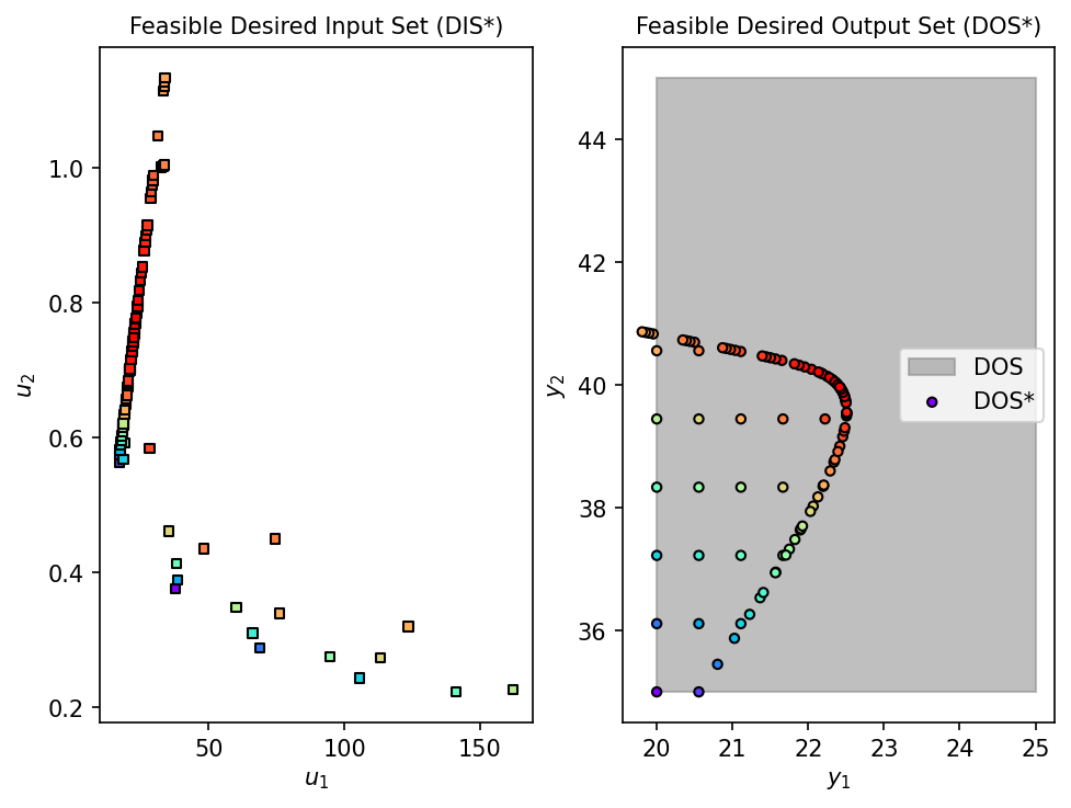
Inverse Mapping Comparison

We now perform NLP-based inverse mapping to find the design region (DIS*) that achieves a desired output specification.

Desired Output Set (DOS):

• Benzene Production: 20–25 mg/h

• Methane Conversion: 35–45%

Constraint: The plug-flow assumption requires a minimum length-to-diameter ratio of 30 to ensure negligible axial dispersion (\(L/D \geq 30\)).

We compare both the surrogate and first-principles models to quantify accuracy and speedup.

Let’s import opyrability’s inverse mapping (NLP-based) module:

from opyrability import nlp_based_approach

# Define DOS, bounds, and constraints
DOS_bounds = jnp.array([[20, 25],    # Benzene [mg/h]
                        [35, 45]])   # Conversion [%]
DOS_resolution = [10, 10]

lb = jnp.array([10, 0.1])    # Lower bounds for L, D
ub = jnp.array([300, 2])     # Upper bounds for L, D
u0 = jnp.array([50, 1])      # Initial estimate

# Plug-flow constraint: L/D >= 30
def plug_flow(u):
    return u[0] - 30.0 * u[1]

constraint = {'type': 'ineq', 'fun': plug_flow}

GP Surrogate Inverse Mapping:

# Inverse mapping with GP Surrogate
print("Running inverse mapping with GP Surrogate...")
start_surrogate = time.time()
fDIS_surr, fDOS_surr, conv_surr = nlp_based_approach(
    jax_surrogate, DOS_bounds, DOS_resolution, u0, lb, ub,
    constr=constraint, method='ipopt', plot=True, ad=True, warmstart=False
)
time_surrogate = time.time() - start_surrogate
print(f"Completed in {time_surrogate:.2f} seconds")

Running inverse mapping with GP Surrogate...
 You have selected automatic differentiation as a method for obtaining higher-order data (Jacobians/Hessian),
 Make sure your process model is JAX-compatible implementation-wise.

  0%|          | 0/100 [00:00<?, ?it/s]

******************************************************************************
This program contains Ipopt, a library for large-scale nonlinear optimization.
 Ipopt is released as open source code under the Eclipse Public License (EPL).
         For more information visit https://github.com/coin-or/Ipopt
******************************************************************************

100%|██████████| 100/100 [01:03<00:00,  1.57it/s]

Completed in 64.38 seconds

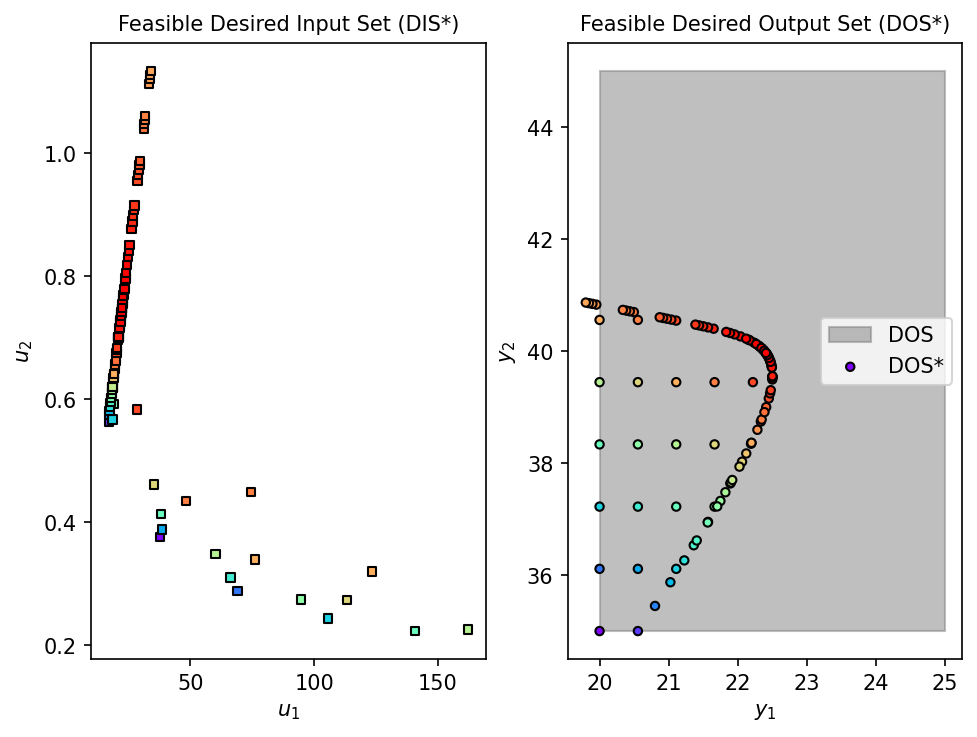
First-Principles Model Inverse Mapping:

# Inverse mapping with First-Principles Model
print("Running inverse mapping with First-Principles Model...")
start_fp = time.time()
fDIS_fp, fDOS_fp, conv_fp = nlp_based_approach(
    dma_mr_design, DOS_bounds, DOS_resolution, u0, lb, ub,
    constr=constraint, method='ipopt', plot=True, ad=True, warmstart=False
)
time_fp = time.time() - start_fp
print(f"Completed in {time_fp:.2f} seconds")

Running inverse mapping with First-Principles Model...
 You have selected automatic differentiation as a method for obtaining higher-order data (Jacobians/Hessian),
 Make sure your process model is JAX-compatible implementation-wise.

100%|██████████| 100/100 [04:11<00:00,  2.51s/it]

Completed in 251.34 seconds

# Overlay plot: Visual comparison of DIS* and DOS* from both approaches
dis_fp = np.array([u for u in fDIS_fp if u is not None])
dis_surr = np.array([u for u in fDIS_surr if u is not None])
dos_fp = np.array([y for y in fDOS_fp if y is not None])
dos_surr = np.array([y for y in fDOS_surr if y is not None])

fig, axes = plt.subplots(1, 2, figsize=(12, 5))

# DIS* overlay
axes[0].scatter(dis_fp[:, 0], dis_fp[:, 1], c='blue', s=60, alpha=0.7, label='First-Principles')
axes[0].scatter(dis_surr[:, 0], dis_surr[:, 1], c='red', marker='x', s=60, alpha=0.9, label='GP Surrogate')
axes[0].set_xlabel('Tube Length [cm]', fontsize=12)
axes[0].set_ylabel('Tube Diameter [cm]', fontsize=12)
axes[0].set_title('Design Space (DIS*) Comparison', fontsize=14)
axes[0].legend(fontsize=11)
axes[0].grid(True, alpha=0.3)

# DOS* overlay
axes[1].scatter(dos_fp[:, 0], dos_fp[:, 1], c='blue', s=60, alpha=0.7, label='First-Principles')
axes[1].scatter(dos_surr[:, 0], dos_surr[:, 1], c='red', marker='x', s=60, alpha=0.9, label='GP Surrogate')
axes[1].set_xlabel('Benzene Production [mg/h]', fontsize=12)
axes[1].set_ylabel('Methane Conversion [%]', fontsize=12)
axes[1].set_title('Output Space (DOS*) Comparison', fontsize=14)
axes[1].legend(fontsize=11)
axes[1].grid(True, alpha=0.3)

plt.tight_layout()
plt.show()

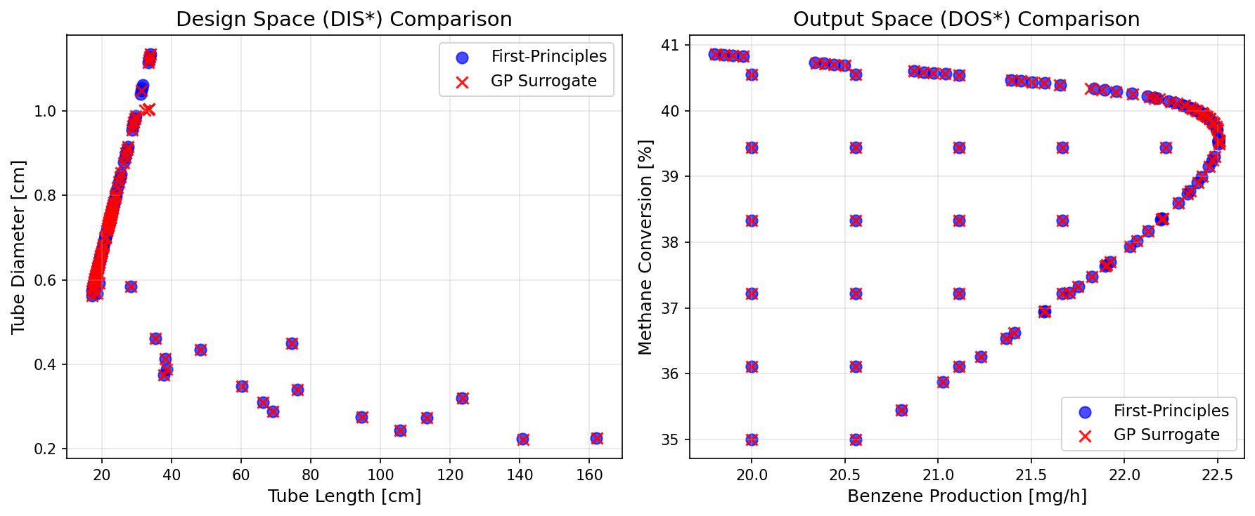
Results Comparison

# Calculate mean design values from DIS*
mean_L_surr = np.mean([p[0] for p in fDIS_surr if p is not None])
mean_D_surr = np.mean([p[1] for p in fDIS_surr if p is not None])
mean_L_fp = np.mean([p[0] for p in fDIS_fp if p is not None])
mean_D_fp = np.mean([p[1] for p in fDIS_fp if p is not None])

print("=" * 60)
print("INVERSE MAPPING COMPARISON")
print("=" * 60)
print(f"\nMean Design Values:")
print(f"  {'Variable':<20} {'First-Principles':>18} {'GP':>18} {'Rel. Error':>12}")
print(f"  {'-'*20} {'-'*18} {'-'*18} {'-'*12}")
print(f"  {'Tube Length [cm]':<20} {mean_L_fp:>18.4f} {mean_L_surr:>18.4f} "
      f"{abs(mean_L_fp - mean_L_surr) / mean_L_fp * 100:>11.4f}%")
print(f"  {'Tube Diameter [cm]':<20} {mean_D_fp:>18.4f} {mean_D_surr:>18.4f} "
      f"{abs(mean_D_fp - mean_D_surr) / mean_D_fp * 100:>11.4f}%")

print(f"\nComputational Time:")
print(f"  First-Principles: {time_fp:.2f} seconds")
print(f"  GP Surrogate: {time_surrogate:.2f} seconds")
print(f"  Speedup: {time_fp/time_surrogate:.1f}x faster")

============================================================
INVERSE MAPPING COMPARISON
============================================================

Mean Design Values:
  Variable               First-Principles                 GP   Rel. Error
  -------------------- ------------------ ------------------ ------------
  Tube Length [cm]                32.1095            32.1554      0.1430%
  Tube Diameter [cm]               0.6913             0.6896      0.2415%

Computational Time:
  First-Principles: 251.34 seconds
  GP Surrogate: 64.38 seconds
  Speedup: 3.9x faster

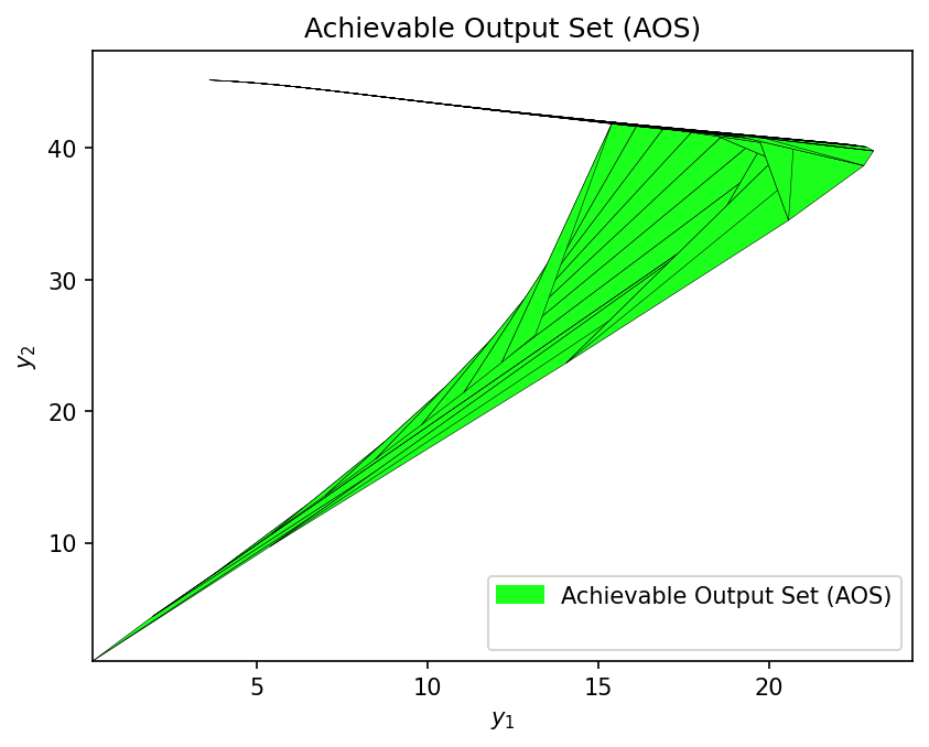
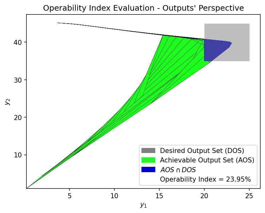
Operability Index Evaluation

Finally, we calculate the Operability Index (OI) using multimodel representation. This measures what fraction of the DOS is achievable given the AIS constraints.

Let’s import opyrability’s multimodel approach and OI evaluation modules:

from opyrability import multimodel_rep, OI_eval

# Define AIS for multimodel representation
AIS_bounds = jnp.array([[10, 300], [0.1, 2]])
AIS_resolution = [10, 10]

# Compute AOS with both models
print("Computing AOS with GP surrogate...")
start_surr_mm = time.time()
AOS_surr = multimodel_rep(jax_surrogate, AIS_bounds, AIS_resolution)
time_surr_mm = time.time() - start_surr_mm
print(f"  Completed in {time_surr_mm:.2f} seconds")

print("\nComputing AOS with first-principles model...")
start_fp_mm = time.time()
AOS_fp = multimodel_rep(dma_mr_design, AIS_bounds, AIS_resolution)
time_fp_mm = time.time() - start_fp_mm
print(f"  Completed in {time_fp_mm:.2f} seconds")

Computing AOS with GP surrogate...

  Completed in 1.51 seconds

Computing AOS with first-principles model...

  Completed in 4.15 seconds

First-Principles Model OI:

OI_fp = OI_eval(AOS_fp, DOS_bounds, plot=True)

GP Surrogate OI:

OI_surr = OI_eval(AOS_surr, DOS_bounds, plot=True)

# OI Comparison Summary
print("\n" + "=" * 60)
print("OPERABILITY INDEX COMPARISON")
print("=" * 60)
print(f"\n  {'Metric':<25} {'First-Principles':>18} {'GP Surrogate':>18}")
print(f"  {'-'*25} {'-'*18} {'-'*18}")
print(f"  {'OI Value':<25} {OI_fp:>17.2f}% {OI_surr:>17.2f}%")
print(f"  {'Multimodel Time [s]':<25} {time_fp_mm:>18.2f} {time_surr_mm:>18.2f}")
print(f"\n  Relative Error in OI: {abs(OI_fp - OI_surr) / OI_fp * 100:.2f}%")
print(f"  Speedup: {time_fp_mm/time_surr_mm:.1f}x faster")

============================================================
OPERABILITY INDEX COMPARISON
============================================================

  Metric                      First-Principles       GP Surrogate
  ------------------------- ------------------ ------------------
  OI Value                              23.95%             24.47%
  Multimodel Time [s]                     4.15               1.51

  Relative Error in OI: 2.15%
  Speedup: 2.7x faster

Conclusions

This example demonstrates that validated GP surrogates can reliably replace computationally expensive first-principles models for operability analysis.

Key Results:

• Surrogate Accuracy: R² > 0.999 on the holdout test set

• Inverse Mapping: <1% relative error compared to first-principles, with ~4x speedup

• Operability Index: ~2% relative error compared to ground truth (OI values are also sensitive to the discretization resolution used)

Workflow Summary:

1. Generate training data from the rigorous model using Latin Hypercube Sampling

2. Train and validate GP models for each output

3. (Optional) Deploy as a JAX function for automatic differentiation

4. Use opyrability functions with the surrogate

The surrogate training is a one-time cost that enables rapid exploration of different DOS specifications or constraint scenarios.